If new data appears on the sheet for the plotted diagram, which needs to be added, then you can simply select a range with new information, copy it (Ctrl + C) and then paste it directly into the diagram (Ctrl + V).

Flash Fill

Suppose you have a list of full names (Ivanov Ivan Ivanovich), which you need to turn into abbreviated names (Ivanov I.I.). To do this, you just need to start writing the desired text in the adjacent column by hand. On the second or third line, Excel will try to predict our actions and perform further processing automatically. All you have to do is press the Enter key to confirm, and all names will be converted instantly. Similarly, you can extract names from email, glue names from fragments, and so on.

Copy without breaking formats

You are most likely aware of the magic autocomplete marker. This is a thin black cross in the lower right corner of the cell, pulling on which you can copy the contents of a cell or a formula to several cells at once. However, there is one unpleasant nuance: such copying often violates the design of the table, since not only the formula is copied, but also the cell format. This can be avoided. Immediately after pulling the black cross, click on the smart tag – a special icon that appears in the lower right corner of the copied area.

If you select the Fill Without Formatting option, Excel will copy your formula without formatting and will not spoil the layout.

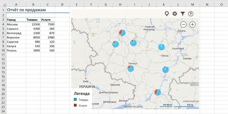
Displaying data from an Excel spreadsheet on a map

In Excel, you can quickly display your geodata on an interactive map, such as sales by city. To do this, go to the Office Store on the Insert tab and install the Bing Maps plugin from there.

After adding a module, you can select it from the My Apps drop-down list on the Insert tab and place it on your worksheet. It remains to select your cells with data and click on the Show Locations button in the map module to see our data on it. If desired, in the plugin settings, you can select the type of chart and colors to display.

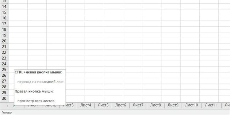
Quick jump to the desired sheet

If the number of worksheets in the file has exceeded 10, then it becomes difficult to navigate them. Right-click any of the sheet tabs scroll buttons in the lower left corner of the screen. The table of contents will appear, and you can jump to any desired sheet instantly.

Convert rows to columns and vice versa

If you have ever had to move cells from rows to columns by hand, then you will appreciate the following trick:

Highlight the range.
Copy it (Ctrl + C) or, by clicking on the right mouse button, select “Copy” (Copy).
Right-click on the cell where you want to paste the data and select one of the Paste Special options – the Transpose icon from the context menu. Older versions of Excel do not have this icon, but you can fix the problem by using Paste Special (Ctrl + Alt + V) and choosing the Transpose option.

Conditional formatting

Something like a chart, only the indicators are not in the next cell, but right in front of the data. This function is turned on to highlight some data in a table.
For example, a teacher in a school makes a table of the average performance of each student. Then the conditional formatting right inside the cells with grades will build a “graph” on which the average scores of each student will be highlighted, for example, from low to high. Or it will highlight the cells in which the average score, for example, is below or above 6. The parameters may be different.
For the function to work, you need to open the “Home” tab, select the field with cells, in the “Styles” tool group find the “Conditional Formatting” iconand choose the appropriate option – it can be a histogram, a color scale, or a set of icons. With the same command, you can independently set the rules for selecting cells.

Sparklines

This tricky word in Excel means a chart created right in a cell and showing the dynamics of row data. It is created like this:

Click “Insert”
Open Sparklines
Select the command “Graph” or “Histogram”
In the window that opens, specify the range with numbers and cells in which sparklines based on these numbers should appear

Macros

And this feature is designed to make life and hard work easier for users. It records the sequence of actions performed, and then performs them automatically, without anyone's participation.
You need to enable the macro by opening the “Developer” tab and finding the “Macro” icon on the toolbar, and next to it – a similar icon with a red circle in the upper left corner. If you need to perform the same action many times, this will start recording a macro, and then the computer will do it by itself.

Forecasts

This option is not advertised by the developers for a reason – it can predict the future! In fact, the function can predict, calculate future values based on already known data that has already been written. Access to it is simple:

Specify at least 2 cells with source data
Open “Data” – “Forecast” – “Forecast sheet”
In the window “Create a forecast sheet” click on the graph or histogram
In the “End of the forecast” area, set the end date, click “Create”

Fill empty list cells

This will save you from monotonous typing of the same phrases into many cells. Of course, you can use the good old copy-paste (copy ctrl + c, paste ctrl + v), but if you need to fill not 10 cells, but, for example, a hundred or two, and the text will be different in places, the next tip will definitely come in handy.
Let's say you have a huge to-do list for the whole week, and you need to set a specific day of the week in front of each task. It is not necessary to prescribe 20 Mondays, Tuesdays and Fridays. In the column, each day of the week is put in the place where the to-do list for that day should begin. It should look something like this:
Next, a column with our days of the week is highlighted, in the “Home” tab, the buttons “Find and select”, “Select a group of cells”, “Empty cells” are pressed. Then, in the first empty cell, you need to put the “=” sign, with the “up” arrow on the keyboard, return to the filled cell (for example, in the table – “Monday”). Press ctrl + enter. Done, now all empty cells should be filled with duplicated data.

Find errors in a formula

Sometimes the formula does not work, but the reason for the “breakdown” is not clear. Sometimes, in order to understand a complex formula (where other functions are taken as an argument to a function) or to find an error in it, you need to calculate only a part of it. Here are two tips:
The formula part is evaluated right in the formula bar. To do this, select the required area and press F9. Everything is simple, but there is one “but”. If you forget to put everything back in place, that is, cancel the calculation of the function and press enter, the calculated part will remain in the form of a number.
Click on “Calculate Formula” in the “Formulas” tab. A window will open where you can calculate the formula step by step and thereby find the moment where the error appears, if there is one, of course.

Smart table

If the user and MS Excel have a different understanding of the concept of a table, this can deprive him of many convenient functions and stretch his work time. Drawn with a pencil or using a border – the program will count it as a regular set of cells. In order for the data to be perceived exactly as a table, this field must be formatted.
It is necessary to select the desired area, in the “Home” tab, click the “Format as table” button. Find a suitable one in the list of different shapes and colors of design options.
Now this is a real table, and if you want to add new formulas to it – you need to insert them border cells, then they will automatically spread to the entire column. Plus, the table header will always be visible when the cursor is scrolled down.

Automatic and manual recalculation

For a book that contains hundreds of complex formulas, you can customize the recalculation at the user's request. For this:

Enter the formula on a blank sheet (so you can check how this example works).
Select a tool: Formulas – Calculation Options – Manual.
Make sure that now after entering data in a cell (for example, the number 7 instead of 1 in cell A2 as in the figure), the formula does not recalculate the result automatically. Until the user presses the F9 key (or SFIFT + F9).

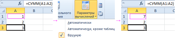
Attention! Fast key F9 – performs recalculation in all formulas of the book on all sheets. A The combination of hot keys SHIFT + F9 – performs recalculation only on the current sheet.

If the sheet does not contain many formulas, the recalculation of which may slow down Excel, then there is no point in using the example described above. But for the future, it is still worth knowing about such a possibility. After all, over time, you will have to deal with complex tables with many formulas. In addition, this function can be turned on accidentally and you need to know where to turn it off for standard operation.

Removing unnecessary columns and rows

This is a fairly common problem when working in Excel. As usual, the user accidentally moves using the hot key combination Ctrl + right or down arrow, pressed accidentally, and is transferred to the end of the sheet, and so it saves the workbook, while significantly making it heavier. This is especially true when a random character, sign, or fill is added to the end of a book.

It is possible to check this option by a characteristic feature, it is a very small slider.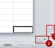

Replace workbook format with * .xlsb

In cases where your work is associated with huge tables and their size reaches large volumes, you should save workbooks in * .xlsb format. This extension is stored as a binary format, a kind of special format for creating and storing your “databases” based on spreadsheets.

When saving in this format, any large file will immediately decrease by 2-3 times, by the way, the speed of calculations will also increase by several orders of magnitude, which will delight you.

Removing excessive conditional formatting

Despite the usefulness of conditional formatting, its overuse can and can lead to problems, your workbook can lag. This can happen, even without your knowledge, just in the process of work you copy cells along with formats and formatting, and this does not go unnoticed, they accumulate imperceptibly and slow down the file.

To remove all that is superfluous, first, select the required range, or you can also the entire worksheet. The next step in the control panel, in the “Home” tab in the “Styles” section, select the item with the drop-down menu “Conditional formatting”, then you need the item “Delete rules” and select the desired deletion sub-item.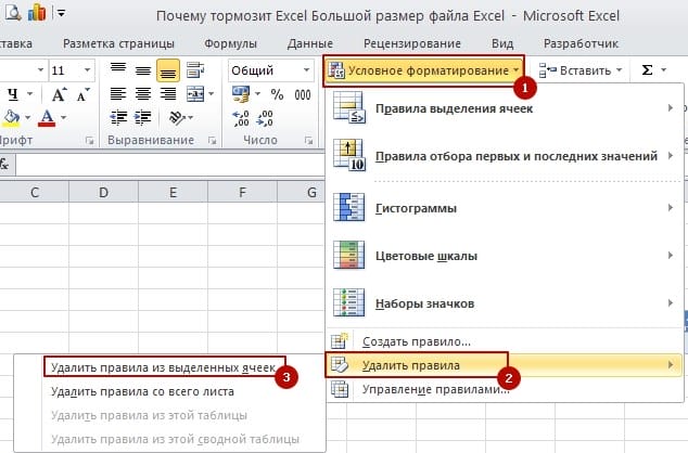

Removing unnecessary data inside the Excel file structure

I can argue that not every user knows that Excel files are a kind of archive and that this file structure began life in 2007. This means that now Excel files can be opened by an archiver such as WinRar. But inside the file there may be files that, in some cases, significantly slow down Excel.

For the procedure to reduce the size, play it safe, and make a backup copy of your file. Then open the file using the context menu, open the file by clicking the right button on the mouse and selecting the “Open with” item and select the archiver program from the available programs. Or, the second option, open the archiver and in the “File” menu click on the “Open inside” item. The result of any of the options will be to open the Excel file as an archive with files and folders.

In the archive, most likely in the “xl” folder, delete the “printerSettings” and “drawings” folders. 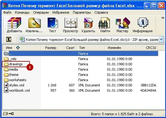After all the torment, we launch the file again and agree to all system indignation with the “Ok” button, the file will be restored and will start.

Please note that if the file contains drawn objects such as buttons or shapes, then you should not delete the entire “drawings” folder, the figures will evaporate with it. It is enough to delete vmlDrawing.vml in the folder, which contains a variety of information and can reach large sizes.

Incorrectly configured print to printer

When you have not set the default printer and the system cannot determine the settings of the current printer, you need to clearly indicate where the printing will take place. If the printer cannot be recognized, replace the device driver.

Sometimes it happens that erasing the printer settings from step 7 can lead to the fact that incorrect printer settings slow down the entire file.

Change Excel version to a later version

Nothing stands still, even our planet, and Excel develops, because there is no limit to perfection. The software product is changing and developing, the software code is being optimized, which allows, sometimes significantly, to increase the productivity of working with tables and calculating formulas, performance can increase up to 20% in newer versions, for example, in 2016 relative to 2007.

Also, quite often there is a situation when Excel 2007 version cannot work with the current file, but in later versions there are no problems and everything works fine.

Upgrade the version, switch to more productive MS Office products, preferably from the 2013 version and above.

Remove extra rows / columns (if the scroll bar is very small)

Most common excel problem I come across. If someone accidentally moved to the end of the sheet (to line number 1 million) and so saved the book. The file size increased immediately. You can reach the end of the table by accident if you press the combination Ctrl + down or right arrow. It happens that there is some random symbol or fill at the end of the book.

The main sign of brakes is the size of the slider, it is very small when the file is saved incorrectly, as in the picture.

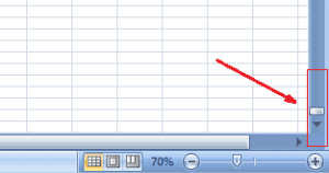
Correct the situation, remove extra rows or columns. Find the last useful cell for you, select the first blank cell after it (or better the first blank row / column after it), press Ctrl + Shift + End. This keyboard shortcut selects cells below the selected row or to the right of the selected column. Right mouse button – Delete – Delete a row or column (usually takes a long time). After deleting, select cell A1 and save the file. The slider should increase.

Remove unnecessary objects

Very often, especially when copying from other files or sites, hidden objects are hidden in tables – pictures, shapes, etc.

To remove such objects, run the macro, press Alt + F11 and copy the text below.

sub DelOb() For Each i In ActiveSheet.Shapes i.Delete Next end sub

Or select and delete objects manually. Go to the menu Home – Editing – Find and Select – Select a group of cells – Objects. Now delete.

Remove unnecessary data in Excel file structure

Even advanced users do not know that an Excel file, as Wikipedia says, is an archive file. Since 2007 release.

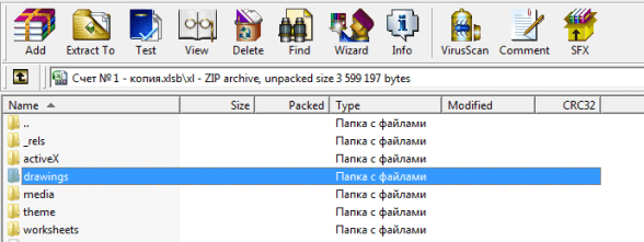
Those. the Excel file is opened, for example, with 7-zip or WinRar archivers. Junk files can be stored inside an open file, which sometimes slows down Excel tenfold.

Shall we remove the inconvenience? First, make a backup copy of the file Then run 7-zip or another archiver, menu “File” – “Open inside”. It is possible to open the file by right-clicking – Open With and selecting the .exe file WinRar or 7-zip.

The archive will open, it is also an Excel file with folders and files.

Find the “drawings” and / or “printerSettings” folders (most likely they will be in the xl folder) and delete them.

We do the same for WinRar.

Then we open the book as an Excel file, he will swear a little, display several system messages that he does not find data, etc. Click OK on all windows, the file will be restored.

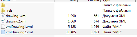
Be careful, if your file contains drawn buttons or other figures, then deleting the entire drawings folder means deleting useful figures.

Therefore, in the folder, delete only the vmlDrawing.vml files, they can accumulate information and weigh up to 100 mb.

Excel slows down – set up pivot tables correctly

If a pivot table refers to a large range of cells, 10,000 or more rows, it stores the calculation results, which can be very large. From this, the entire excel book slows down, of course. To eliminate this reason, right-click on the pivot table – Pivot table options – Data tab – uncheck the Save original data with file checkbox.

That will reduce the file by almost half.

Change the file format to .xlsb

If you work with huge tables and your files are larger than 0.5 mb in weight, then it is better to save such books in .xlsb format. The binary format of an Excel workbook, i.e. a special format for creating a “database” based on spreadsheets. If you save a large file in this format, the weight of the book will be reduced by two to three times. Calculations to a file will also be faster, in some cases 2 times faster.

Unrecognized printer installed

If you do not have a printer defined on your computer, i.e. there is no default printer, then go to devices and printers and change the default printer to any other (even if there is no physical printer), if there is a printer, it is better to change the firewood.

It happens that even when deleting printer settings from step 5, the printer settings slow down the file.

Excel tip. Hotkeys

Tip number two follows from the first – learn hotkeys. There are not so many useful hotkeys, so after learning 10-20 shortcuts, you will quickly feel the difference in the speed of work.

“Nice advice!” – you object. – “And how to teach them? Stand on a stool in front of colleagues and recite like poetry?”

Not. Of course it's not like that. try to find your own way of learning keyboard shortcuts. What can be done for this?

For example, you can take a list of hotkeys and select 3-5 of the most used functions. Try to work them out, practice how they work. Get used to hitting them when you need them. Over time, the fingers themselves will lie on the keyboard so that you can quickly and conveniently switch between sheets. Once you have learned these, move on to the next, and then again and again.

Excel tip. Functions and their combinations that must be mastered

It may sound trite, but you need to know the functions to work faster in Excel. I am sure that you, my dear reader, are fluent in Excel functionality and can make very cool reports and calculations in Excel. However, it is possible that not all functions are subject to you, and there is something to strive for.

Also, each function can have many uses. So, for example, do you know that the SUM function can sum up values from different sheets of your workbook without having to select each of them separately? Those.

Instead of the formula

SUM (Sheet1! A1; Sheet2! A1; Sheet3! A1; Sheet4! A1; Sheet5! A1; Sheet6! A1; Sheet7! A1; … SheetN! A1)

The formula will look like

SUM (Sheet1: SheetN! A1)

What is all this for? In addition to the rich functionality of Excel, which is in its standard formulas, there are many combinations, the knowledge of which allows you to solve non-standard tasks. So, Excel does not have the MINESLI function at all. Yes, there is SUMIF, COUNTIF, but MINESLY did not. Also MAXESLI, MEDIANESLI, etc., but all this is solved by using the functions of the areas. You may have seen when a formula is wrapped in curly braces.

Some functions work fine only in conjunction. I'm talking about INDEX and SEARCH. It would seem that they are stupid functions separately, but together they give excellent functionality.

In general, ladies and gentlemen, I recommend that you learn formulas and all sorts of tricks with these formulas.

What is needed for this? For example, subscribe to our group in and wait for the release of new posts.

Excel tip. Structure and formatting in files

If you have come across the principles of modeling, then you obviously know that in order to avoid mistakes, it is enough to put things in order in your calculations.

Confusing calculations, clutter and inconvenient navigation lead to the fact that even the author himself begins to wander in the file.

How can this be avoided? Here are some tips:

Format the file. Let you have the same number of decimal places, the same font throughout your document, and a limited color palette. I like to use palettes of the same color but different tones (cyan, blue and dark blue). Looks very stylish.
Separate input data, calculations and results. This is not always necessary, but when there is a lot of data, the presence of a pivot plate simply saves.
Do the same formulas by column or row. agree not very correctly when the same indicator in different periods is considered differently. At the same time, this is usually not visible until you look at the formula. but you can also forget about the honor.
Try to avoid circular references and links to external files. Usually they give different results on different computers. There was a case when the error when updating external links was more than 7 zeros. Ay!
Simplify and save space. Excel allows you to create as many rows and columns as you like. In my 10 years of working with the program, I have never used the sheet completely. It is unlikely that you will succeed, so do not fence complex formulas. Better do the calculation in a few steps.

Sources used and useful links on the topic: https://Lifehacker.ru/uskorennaja-rabota-v-excel/ https://zen.yandex.ru/media/id/5a323345780019a66a1ed2c7/uskoriaem-rabotu-v-excel-poleznye- sovety-funkcii-bystrye-klavishi-5ac7331bdcaf8e9121c8583b https://exceltable.com/formuly/avtomaticheskiy-pereschet-formul http://topexcel.ru/pochemu-tormozit-excel-12-sposobov-uluchsit-fajot https://excelworks.ru/2015/03/18/tormozit-excel/ https://finversity.ru/tryuki-excel/kak-rabotat-v-excel-v-3-5-raz-byistree.html

Post source: lastici.ru